📚

All Subjects

♾️

AP Calc

🐶

Unit 8

Unit 8 Overview: Applications of Integration

8 min read•june 18, 2024

Kashvi Panjolia

Anusha Tekumulla

AP Calculus AB/BC ♾️

279 resources

See Units

In this unit, you’ll learn how to find the average value of a function, model particle motion and net change, and determine areas and volumes. Specifically, you should develop an understanding of integration that can be transferred across many other applications. You'll start to see how integration is useful in the fields of physics and engineering, and exercise your drawing skills as you draw sketches to visualize 2D and 3D shapes. With integrals, you won’t have to use any of the Riemann sums you learned earlier in the year. It is crucial to understand the general steps for solving each problem in this unit. This unit should be about 10-15% of the AP Calculus AB Exam or 6-9% of the AP Calculus BC Exam.

8.1 Finding the Average Value of a Function on an Interval

In calculus, the average value of a function is the value that the function would take at a single point if the area under the curve were equal to the area of a rectangle with the same width and height as the curve. In other words, it is a way to measure the "center of mass" or "balance point" of a function.

The average value of a function f(x) over the interval [a,b] is given by the formula:

To find the average value of a function, you can first set up the definite integral for the function over the interval of interest. Then, you can evaluate the definite integral using the appropriate techniques, such as substitution.

8.2 Connecting Position, Velocity, and Acceleration of Functions Using Integrals

If you have taken or are taking a physics course, then you already know what position, velocity, and acceleration are. If you haven't heard these terms before, you only need to know that position is where an object is at a moment in time, velocity is the rate of change (read as derivative) of the position as a function of time, and acceleration is the rate of change (read as derivative) of velocity as a function of time.

Definite integrals can be used to calculate the displacement and total distance traveled for a particle in linear motion over a certain interval of time.

Displacement is a vector quantity that represents the change in position of an object. It can be found by taking the definite integral of the velocity function with respect to time. This is because velocity is the rate of change of position, and the definite integral of a rate of change is the change itself.

On the other hand, the total distance traveled is a scalar quantity that represents the total distance covered by the object, regardless of its final position. It can be found by taking the definite integral of the speed function with respect to time. This is because speed is the magnitude of the velocity and the definite integral of a scalar function represents the accumulated change in the function over a certain interval.

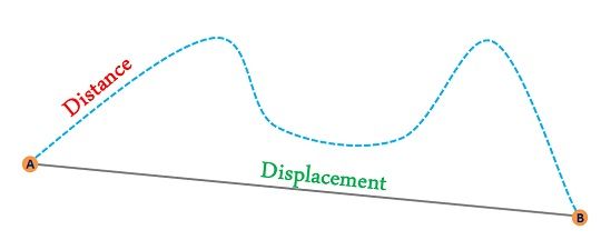
Image courtesy of Key Differences.

8.3 Using Accumulation Functions and Definite Integrals in Applied Contexts

The definite integral, as you already know, is a fundamental concept in calculus that allows us to calculate the accumulated change of a function over a certain interval. It can be used to express information about accumulation and net change in many applied contexts, such as physics, engineering, economics, and many others.

Integration can be used to calculate the total cost of producing a product, the total revenue or cost of a company, the total distance covered by a moving object, and much more. You will be asked on the AP exam to use definite integrals to compute an answer to many real-world scenarios, such as the amount of water leaking from a tank, through word problems.

8.4 & 8.5 Finding the Area Between Curves Expressed as Functions of x and y

Finding the area between two curves using integrals involves calculating the definite integral of the difference between the two functions over a given interval. The process is similar whether the curves are functions of x or y.

When the curves are functions of x, we need to find the definite integral of the difference between the two functions, f(x) and g(x), with respect to x over the interval [a, b]. The definite integral representing the area between the curves is given by:

This definite integral represents the area between the two curves as a function of x from x=a to x=b. When the curves are functions of y, we perform the same subtraction, but this time we subtract the left from the right function to obtain a positive area.

8.6 Finding the Area Between Curves That Intersect at More Than Two Points

Calculating this type of area is similar to the topic discussed above, but with a few extra steps since there are more points of intersection. When two curves intersect at multiple points, the area between them can be found by calculating the sum of the areas of the multiple regions created by the intersection points. The process for finding the area between two curves that intersect at multiple points is similar to finding the area between two curves that do not intersect, but it involves breaking the interval of integration into smaller intervals.

The process of finding the area between two curves that intersect at multiple points is as follows:

Find the points of intersection: Find the x or y values of the points of intersection, where the two curves meet. You can do this by setting the two functions equal to each other.
Divide the interval of integration: The next step is to divide the interval of integration into smaller intervals between the points of intersection.
Evaluate the definite integral over each interval: For each interval, find the definite integral of the difference between the two functions over that interval, as we learned in the last topic.
Sum up the areas: Sum up the areas of the regions created by the intersection points.

Consider the graph of two functions below. The two functions intersect at three points and create two equal sections of area between them.

You can find the area of both sections by finding the points at which the functions intersect when you set them equal to each other. Then, create a definite integral for the area of one of the two sections and multiply that area by 2 to obtain the area for both sections.

8.7 & 8.8 Volumes with Cross Sections

Finding the volume of a function using a square or rectangular cross-section and integrals involves using the method of slicing, where the function is represented as a solid of revolution formed by rotating a two-dimensional region about an axis to create a three-dimensional shape.

The process for finding the volume of a function using a square or rectangular cross-section is as follows:

Identify the region of interest: The first step is to identify the region of interest in the xy-plane, which is the region that will be rotated to form the solid. You can do this by finding the limits of integration.
Choose an axis of rotation: The next step is to choose an axis of rotation. You will be rotating objects mostly along the x- or y-axis.
Choose a cross-section: The third step is to choose a cross-section. The square or rectangular cross-section is chosen, which is perpendicular to the axis of rotation.
Divide the region of interest into small rectangular slices by adding the width of the cross-section.
Find the area of each slice: The area of each slice is obtained by multiplying the length of the rectangle by its width (the function value).
Integrate over the interval: Add up all the areas over the interval of interest. The definite integral of the areas over the interval of interest represents the total volume of the solid.

The definite integral representing the volume of a function using a square cross-section is given by:

∫ (f(x))^2 dx

The function is squared here because that is the formula for the area of a square (squaring the side length). For a rectangle, the formula for the volume becomes

∫ (f(x))*w dx

The area of a triangle is 1/2bh, so applying that to the basic integration formula we have been using, we get

∫ (1/2)*(f(x))*w dx

The area of a semicircle is found by halving the area of a circle. Using (1/2)πr^2, the formula is

∫ (1/2)(π(f(x))^2)*w dx

As you can see, the volume of a cross-section is determined by the shape of a cross-section. You will likely need to create quick sketches to visualize these 3D shapes, so make sure your pencils are sharpened. ✏️

8.8 & 8.9 Volume with Disc Method

The disc method is a method used in calculus to find the volume of a solid of revolution obtained by rotating a two-dimensional region about an axis. It is based on the idea of cutting the solid into thin disks parallel to the axis of rotation and finding the volume of each disk.

The disk method is used to find the volume of a solid of revolution when the cross-section of the solid is a disk (circular) shape, so we use the formula for the area of the circle and apply it to our integral:

∫ π*(f(x))^2 dx

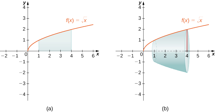
$https://math.libretexts.org/@api/deki/files/12439/6.2.5.png?revision=1$

Image courtesy of MathLibreTexts.

These same concepts are used to rotate a function around a horizontal or vertical line other than the x-or y-axis, but with some additional steps.

8.11 & 8.12 Volume with Washer Method

The washer method is a method used to find the volume of a solid of revolution obtained by rotating a two-dimensional region about an axis. It is similar to the disk method but instead of using disks to find the volume, it uses "washers" which are ring-shaped objects with an inner and outer radius. The washer method is used when the cross-section of the solid is not a disk shape but a ring shape.

Instead of a disk, we find the area of the washer cross-section. This area is given by π*(R^2 - r^2), where R is the outer radius and r is the inner radius of the washer. Then, we integrate as before to find the total volume of our shape. Below is the formula for the washer method:

As with the disc method, functions can be revolved using the washer method around axes that are not the x- or y-axes with a few additional steps involved.

8.13 The Arc Length of a Smooth, Planar Curve and Distance Traveled (BC Only)

In order to find the total distance traveled of an object, we need to calculate the arc length of the velocity function for that object. Arc length is a measure of the distance along the curved path of a function, such as a circle or a parabola. In calculus, the arc length of a function can be calculated using integrals. There is only one formula you need to memorize to calculate the arc length of a curve in the Cartesian plane:

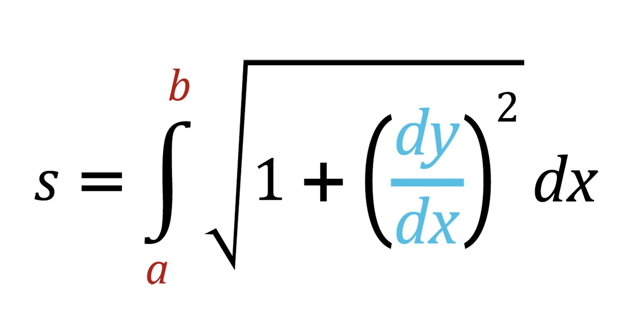
Image courtesy of Chegg.

This formula states that you need to find the derivative of the function, square it, add 1, take the square root, then integrate that over your interval.