📚

All Subjects

🤑

AP Micro

🏋🏼‍♀️

Unit 3

Unit 3 Overview: Production, Cost, and the Perfect Competition Model

7 min read•june 18, 2024

Maria Guerra

dylan_black_2025

AP Microeconomics 🤑

95 resources

See Units

Unit 3 Overview: Production, Cost, and the Perfect Competition Model

Welcome to Unit 3 of AP Micro! I cannot express this any more than I will here: UNIT 3 IN AP MICRO IS THE MOST IMPORTANT UNIT OF ALL OF THEM!!!!! This unit is the foundation of at minimum, units 3 (duh), 4, and 5. Without Unit 3, units 4 and 5 just fall apart. Take ALL the time you need on this unit. Seriously. If you need to read these guides 100 times to understand, that's fine! And get excited, because this is where the fun starts!

Welcome to the bread and butter of microeconomics! Unit 3 marks the introduction of the producer side of Micro. In units 1 and 2, we spoke quite a bit about consumers with utility maximization and supply and demand, but producers really got relatively pushed to the side besides brief discussions here and there and discussions of the supply curve. In this unit, we put producers in the forefront.

We'll begin by looking at how production actually works and how we as economists measure how a firm producers. This involves some more marginal analysis and understanding yet another example of the law of diminishing marginal returns.

After that, we'll look at cost structures, employing more marginal analysis and a bit of math to understand how firms costs' change with quantity. This includes understanding total costs, fixed costs, variable costs, and per-unit costs along with marginal cost.

The next piece of the puzzle is understanding revenue and profit. The fundamental question a firm is always asking is how they can maximize their profit. We'll uncover a rule for how a firm maximizes their profit by relating marginal revenue to marginal cost (no spoilers though!).

Every time you think about the Law of Diminishing Marginal Returns, you gain slightly less knowledge than the last time you thought about it. See what I did there?

Finally, we'll put all these pieces together to discover our first market structure: perfect competition. From this, we can understand how a theoretically perfect market acts - one with many sellers and buyers and easy entry with identical products.

Let's break down each unit and the broad motivation questions that will follow us through Unit 3:

Unit 3.1: The Production Function

Unit 3.1 gets right to work defining how firms produce goods using the factors of production, land, labor, and capital. This section defines total product, marginal product, and average product and discusses how each of these measures relate to each other graphically and mathematically.

You'll also learn how inputs scale to outputs by discussing returns to scale. When a firm doubles its inputs, what happens to output? Does it exactly double? More than double? Less than double? Understanding returns to scale

Graphs Learned:

None...

Unit 3.2: Short-Run Production Costs

This unit is one of the most important in unit 3! This unit is all about how costs change depending on quantity in the short-run. The short-run is the period in which at least one of our inputs are fixed. This is important since in the long-run, costs look different because we can always minimize our costs!

We start by defining the difference between variable costs and fixed costs and using them to calculate total cost using the formula TC = FC + VC. The main distinction is that fixed costs are just that - fixed! They do not change with quantity. If we produce 10 units or 100 units, fixed cost is the same.

We then take a look at our per-unit cost curves, or average cost curves, which are our total cost, variable cost, and fixed cost per quantity. Thus, average total cost = TC / Q, and so on. These relate to our marginal cost, the additional cost of producing one more unit.

Using graphs like the one below and some tables, we'll understand all about how costs work in the short-run, giving us half of what we need to model a market. Next, we need revenue.

Unit 3.3: Long-Run Production Costs

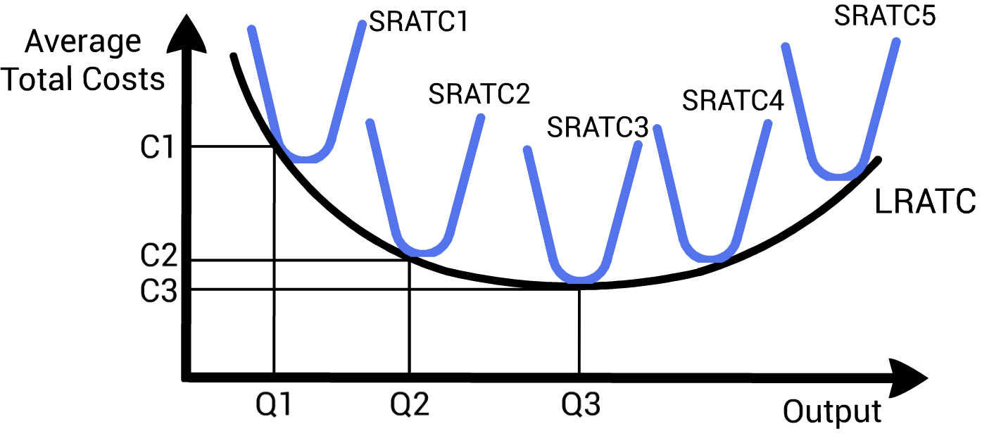
Before we jump into revenue, we'll take a look at what production costs look like in the long-run, when all inputs are variable. When inputs are variable, a firm can always adjust to minimize costs regardless of what short-run average total cost curve it's on. Repeating this, we will form a long-run average total cost curve that represents the lowest cost achievable at each output. This will help us model economies of scale, in which as we scale up, costs in the long-run decrease. We'll also look at diseconomies of scale, which is the opposite. After you understand short-run and long-run costs, you're ready to put them to work in understanding revenue and profit in 3.4!

Unit 3.4: Types of Profit

Now that we understand costs, let's break down what profit is. In economics, we have revenues, or gains, and costs. Profit is the excess revenue that a business gets to keep. Mathematically, this is represented as Profit (oftentimes notated as π) = TR - TC. However, there are two types of profits we'll discuss.

Accounting profit is the profit when just money on paper is looked at. This is the profit you're most likely already familiar with. If you spend $5 opening a lemonade stand and make $30 in revenue, your accounting profit is $25.

However, in economics (as opposed to business and accounting), we look at the implict or opportunity costs as well! This is how we define economic profit. Economic profit is the total revenue minus the accounting costs and opportunity costs. For example, if your family offered you $10 not to open the lemonade stand at all but you did anyway, your total costs are not $15, meaning your economic profit is only $15.

We'll also discuss the difference between positive profits, when TR > TC, losses, when TR < TC, and normal profits, when TR = TC.

We also discuss marginal revenue, which is the additional revenue gained by producing one more unit.

Unit 3.5: Profit Maximization

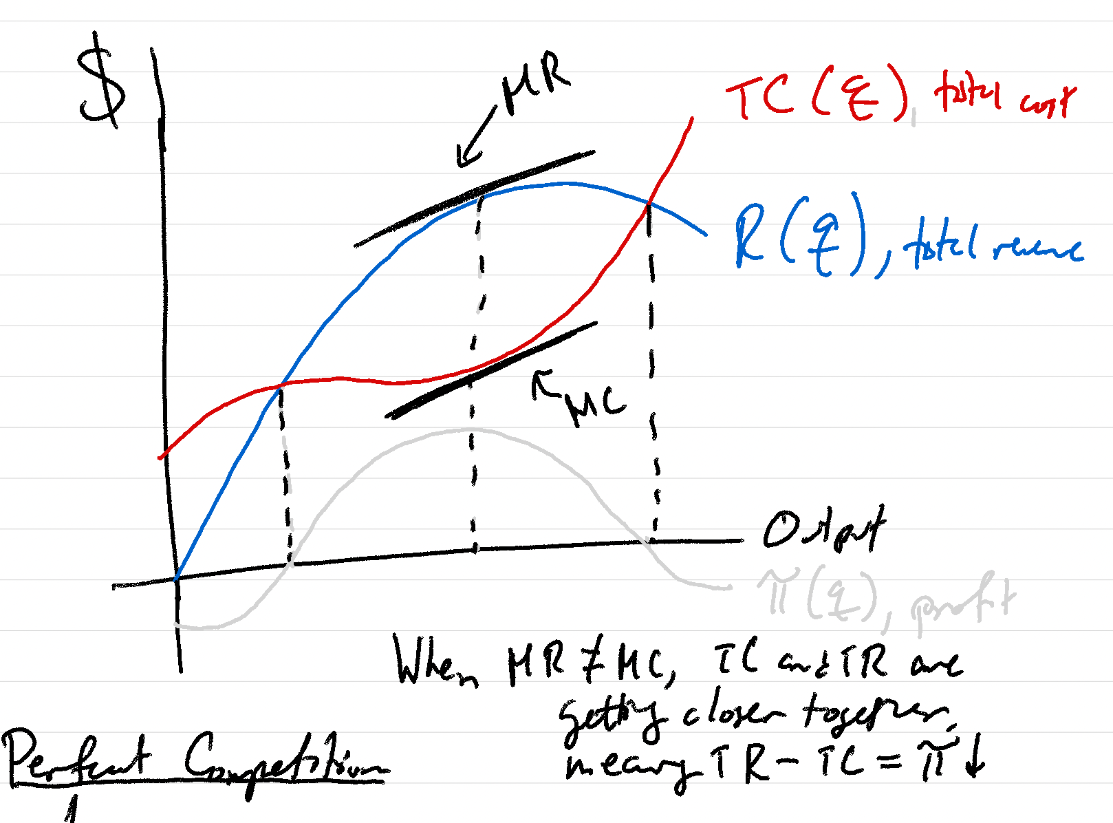
Firms have one primary goal in mind when they are producing: how do I maximize my profits? This is not as simple as maximizing revenue, because costs could be really high as well! The profit maximizing rule for a firm is to always produce where MR = MC. This is because you earn all available profits while not overshooting and incurring additional costs. The last four units have led up to this! We now know, as a firm, how much to produce to maximize our profit.

Unit 3.6: Firms' Short-Run Decisions to Produce and Long-Run Decisions to Enter or Exit a Market

Sometimes, a firm needs to know when to begin production (enter a market), or cease all production (exit a market). Now that we understand profit, we know what a firm does, and therefore we can understand if that quantity is viable for a firm. We discuss the shut down rule, which states that a firm should not produce unless it can cover its variable costs. If it can't (which happens in perfect competition when P < AVC at MR = MC), we are better off taking the hit on our fixed costs (which are sunk in the short run), and producing nothing.

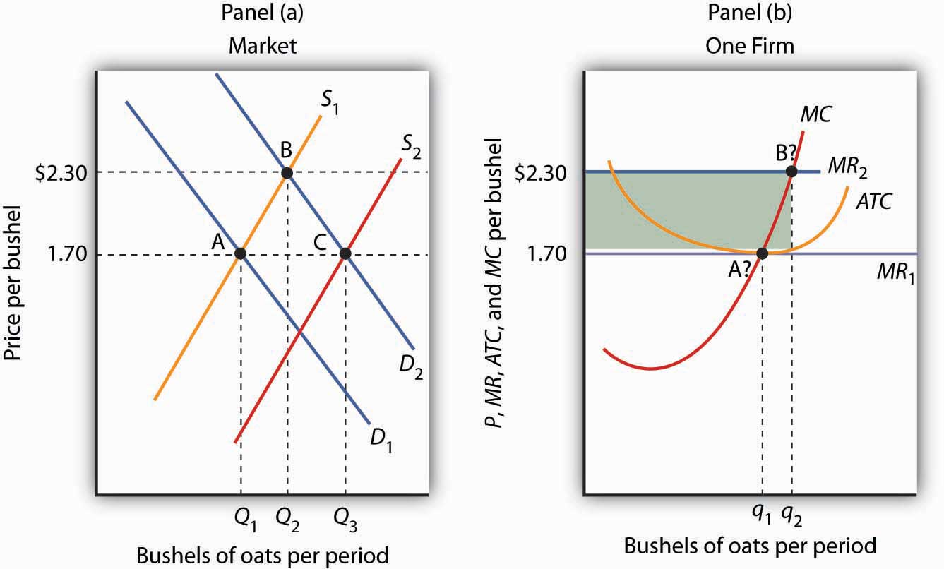
We'll also better understand how markets act in the long run, with firms exiting or entering depending on the profits earned in the short-run. In the long-run, all costs are variable, so a firm won't produce in the long run if it isn't making at least a normal profit. Thus, in the long-run, firms leave when profits are negative, and enter when profits are positive. This leads to a long-run adjustment in the long-run that equilibrates the market where all firms make a normal profit:

Unit 3.7: Perfect Competition

At long last! We've learned all about how producers function, how their costs work, how their revenues and profits work, how to maximize said profits, and how to know whether we should produce in the short-run and long-run! This means we're finally ready to put together perfect competition, our first market structure in AP Microeconomics.

In perfect competition, there are many identical firms all competing at a constant market price. Perfect competition also is a market structure with low barriers, meaning in the long run anyone can enter or exit the market. By using everything we've learned, we can graph what a perfectly competitive market and firm look like side by side:

Perfectly competitive firms are price takers, which mean they cannot charge a price higher than the market equilibrium price. This is because they have no market power. This will be contrasted with unit 4's structures, which are imperfectly competitive, but until then, you've done it! You've learned everything you need in unit 3 of Microeconomics. You can now explain perfect competition and all its associated cost curves!

Browse Study Guides By Unit

💸Unit 1 – Basic Economic Concepts

📈Unit 2 – Supply & Demand

🏋🏼‍♀️Unit 3 – Production, Cost, & the Perfect Competition Model

3.0Unit 3 Overview: Production, Cost, and the Perfect Competition Model