9.3 Justifying a Claim About the Slope of a Regression Model Based on a Confidence Interval
4 min read•june 18, 2024
Jed Quiaoit
Josh Argo
AP Statistics 📊
265 resourcesSee Units
A couple reminders from earlier sections:
- A confidence interval gives us a good prediction on what the slope of the true linear regression model for a population’s set of data by giving us a range of values to predict.
- The point estimate for the slope of a regression model is the slope of the line of best fit, b.
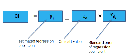
- For the slope of a regression model, the interval estimate is b + t* (SE of b).
In this section, we'll answer a burning question in this unit: how can we justify (or dispute) a claim about a linear regression model using this data? 🤔

One of the important things about a confidence interval that we must set is the confidence level. Remember that this confidence level reflects the percentage of confidence intervals that would contain the true value we are aiming towards (in this case slope) if we were to take several unique samples of our given sample size. 👍
For example, if we were to construct a 95% confidence interval to estimate the slope of a linear regression model, this means that if we were to create several random samples of the same size, from the same population, 95% of the resulting confidence intervals would contain the true slope of the population regression model.
Confidence Interval
A confidence interval is going to provide us with plausible values for our slope. For instance, if our confidence interval for the slope is (1.35, 2.7), we can be pretty certain that our correlation is positive and our slope is somewhere between 1.35 and 2.7.
Our interpretation of this would state something like: ➕
- We are 95% confident that the true slope of the regression line showing the correlation between variable A and variable B is somewhere between 1.35 and 2.7.
- In repeated random sampling with the same sample size, approximately 95% of confidence intervals created will capture the slope of the regression model, i.e., the true slope of the population regression model.
This is a very similar interpretation to what we used in Units 6 and 7, but altered to estimate the true slope instead of true mean or proportion.
Another thing worth noting is that the width of the confidence interval is going to decrease as the sample size increases. This is because an increased sample size decreases our standard error. Also, as the confidence level increases, the width of our interval will increase.
Justifying a Claim
If we are seeking to justify a claim about correlation with our confidence interval for slopes, we should be seeking to determine if 0 is contained in our interval. 0️⃣
If 0 is contained in our confidence interval, it is definitely plausible that 0 is the slope of our least squares regression model. If 0 is the slope, there essentially is no linear correlation.
For example, if we use our interval from the previous example (1.35, 2.7), this tells us that the two variables of interest ARE correlated because there 0 is not contained in our interval so we can be 95% confident (or whatever confidence level) that our slope is positive and our variables have a positive correlation of some sort.
Example
The most likely type of question you would see on linear regression on the AP exam would involve a computer output. Using a computer output, we'll interpret what our confidence interval would look like. We also need a sample size to compute our t score, so let’s assume our sample size is 40 for our scatterplot and a 95% confidence level. 🖥️
First, we would need to compute our t score by doing invT based on 38 degrees of freedom (n - 2). The other aspects of our confidence interval are already in our problem. Our t-score for a 95% confidence interval comes out to be 2.02.
Our confidence interval would be 0.4482.02(0.6565), which is the slope estimate plus/minus (t score)(standard deviation/error). Be careful not to use the t score given in the table. That is the t score for our sample not for the desired confidence interval.
This would yield a final example of (-0.87813, 1.77413). Since 0 is contained in this interval, we do not have evidence that there is a linear correlation (which is also evident by the low R2 value and subsequent low r value (0.176).
🎥 Watch: AP Stats Unit 9 - Inference for Slopes
Browse Study Guides By Unit
👆Unit 1 – Exploring One-Variable Data
✌️Unit 2 – Exploring Two-Variable Data
🔎Unit 3 – Collecting Data
🎲Unit 4 – Probability, Random Variables, & Probability Distributions
📊Unit 5 – Sampling Distributions
⚖️Unit 6 – Proportions
😼Unit 7 – Means
✳️Unit 8 – Chi-Squares
📈Unit 9 – Slopes
✏️Frequently Asked Questions
📚Study Tools
🤔Exam Skills

Fiveable
Resources
© 2025 Fiveable Inc. All rights reserved.