4.2 Estimating Probabilities Using Simulation

5 min read•june 18, 2024

Kanya Shah

Jed Quiaoit

AP Statistics 📊

265 resources

See Units

A simulation is a useful tool in statistics that allows us to anticipate patterns in data by generating synthetic data based on certain assumptions or models. Simulations can be used to explore the behavior of a statistical model or process over a range of scenarios, and can provide insights into the likely patterns that will emerge in real-world data. In this section, we'll make sure you know how to conduct or come up with a simulation with several trials and calculate probabilities from the resulting data. 🌎

Simulation Time!

Simulations are examples of random processes, which generate results that are determined by chance. These processes yield results, also known as outcomes, from trials. Combining a bunch of these overall outcomes leads to what we call an event. 🎲

One example that could clarify the difference between an outcome and an event is the example of die rolling:

Rolling a particular value on a six-sided number cube is one of six possible outcomes, as in getting a 1, 2, 3, 4, 5, OR 6, illustrates an outcome.
When rolling two six-sided number cubes, an event would be a sum of seven. The corresponding collection of outcomes would be (1, 6), (2, 5), (3, 4), (4, 3), (5, 2), and (6, 1), where the ordered pairs indicate (face value on one cube, face value on the other cube).

Where do simulations come in, then? 📶

Large Numbers Have Laws, Too!

As a refresher, probability is defined as a numerical outcome between 0 and 1 of a chance process. Here's the new idea: probability also describes the proportion of times the outcome would occur in a very long series of repetitions. Chance behavior is unpredictable in the short run but has a regular and predictable pattern in the long run, which is described by the law of large numbers.

The law of large numbers states that simulated (empirical) probabilities tend to get closer to the true probability as the number of trials increases. 🏗️

Here are a couple of applications of the law in common probabilistic examples:

Flipping a coin: If you flip a coin a large number of times, the law of large numbers states that the simulated probability of getting heads will tend to approach the true probability of getting heads (which is 0.5) as the number of flips increases. For example, if you flip a coin 10 times and get 6 heads, the simulated probability of getting heads is 0.6. If you flip the coin 100 times and get 50 heads, the simulated probability of getting heads is 0.5. As you can see, the simulated probability gets closer to the true probability as the number of flips increases.
Rolling a die: The law of large numbers can also be applied to the rolling of a die. If you roll a die a large number of times, the simulated probability of rolling a particular number (such as a 6) will tend to approach the true probability of rolling that number (which is 1/6) as the number of rolls increases.
Spinning a roulette wheel: The law of large numbers can also be applied to the spinning of a roulette wheel. If you spin the wheel a large number of times, the simulated probability of the ball landing on a particular number (such as 25) will tend to approach the true probability of the ball landing on that number (which is 1/38) as the number of spins increases.

Rinsing & Repeating

To give a simpler definition of the section opener above, a simulation is a way to model random events, such that simulated outcomes closely match real-world outcomes. All possible outcomes are associated with a value to be determined by chance.

In a simulation, all possible outcomes are associated with a value that is determined by chance. For example, in a simulation of rolling a die, there are six possible outcomes (rolling a 1, 2, 3, 4, 5, or 6), and each outcome is associated with a certain probability (1/6 for each outcome). 🤷‍♂️

To conduct a simulation, we typically repeat the process a large number of times (known as trials) and record the counts of the simulated outcomes. We can then use these counts to calculate the simulated probability of each outcome, and compare these probabilities to the true probabilities that we expect to see in the real world.

Here's the process of conducting a simulation in bullet point terms: 🚴

Describe how to use a chance device to imitate one trial (repetition) of the simulation. State what you’ll record at the end of each trial.
Perform many trials of the simulation.
Use the results of your simulation to answer the question of interest.

🎥 Watch: AP Stats - Probability Rules and Random Variables

Courtesy of AHS Weebly

Practice Problem

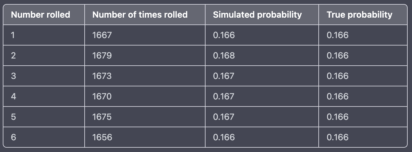
A statistics professor is interested in studying the behavior of a six-sided die, and decides to conduct a simulation to explore the probabilities of rolling different numbers. To do this, the professor sets up a computer program to simulate the rolling of a die 10,000 times, and records the outcomes of each roll.

The professor then calculates the simulated probability of rolling each number, and compares these probabilities to the true probability of rolling each number (which is 1/6 for each number). The results of the simulation are shown in the table below:

Based on the results of the simulation, the professor makes the following conclusions:

The simulated probabilities of rolling each number are very close to the true probabilities.

The simulated probabilities of rolling each number are not significantly different from one another.

Write a brief summary explaining the professor's conclusions and the statistical evidence that supports them.

Answer

The professor concludes that the simulated probabilities of rolling each number are very close to the true probabilities, and that the simulated probabilities of rolling each number are not significantly different from one another, based on the statistical evidence provided in the simulation results.

One piece of evidence that supports these conclusions is the fact that the simulated probabilities of rolling each number are all very close to the true probability of 1/6. This suggests that the simulation is producing outcomes that are consistent with the probabilities that we would expect to see in the real world.

Another piece of evidence that supports these conclusions is the fact that the simulated probabilities of rolling each number are not significantly different from one another. This suggests that the simulation is not producing outcomes that are biased towards any particular number, and that all of the numbers are equally likely to be rolled.

Overall, the statistical evidence suggests that the simulation is producing outcomes that are consistent with the true probabilities of rolling each number, and that the outcomes are not significantly different from one another. This supports the professor's conclusions about the behavior of the die.

Browse Study Guides By Unit

👆Unit 1 – Exploring One-Variable Data

✌️Unit 2 – Exploring Two-Variable Data

🔎Unit 3 – Collecting Data

🎲Unit 4 – Probability, Random Variables, & Probability Distributions

4.0Unit 4 Overview: Probability, Random Variables, and Probability Distributions

4.1Introducing Statistics: Random and Non-Random Patterns?

4.2Estimating Probabilities Using Simulation

4.3Introduction to Probability

4.4Mutually Exclusive Events

4.5Conditional Probability

4.6Independent Events and Unions of Events